I keep coming back to these ideas
I did mention some of it a while back, but also I am re-reading “Thinking in Systems” by D. H. Meadows.
Well, I still truly do NOT know how I will go about it (if and when I decide to put more efforts into coding these things), but for the time being, I thought I’d run some extremely simplistic - and absolutely incorrect and personal - approach to it all.
About “stocks”
One topic that appears a bit in the referenced book is the idea of stock, as in “storage buffers” of “flows” (that’s how I understood it anyway). Think bathtub, faucet and drain.
So how about this for a simplistic idea. Two companies compete to “grow” with two different HR policies, one more focused on improving hiring, the other on retention.
Both have supposedly “good policies” towards an objective of growth, in that their respective policies seem “positive”, more “in-flow” that “out-flow”.
Now (and again, this is stupid as a model I suppose, it is just me warming up to the concepts), what if there was a limited “pool” of potential employees, a “general population” from which to hire from (or “fire into”).
I coded a very very simplistic (and absolutely zero-optimized, nor probably even quite correct) thing to represent this, which looks at the “current stock” of each company (and well, the general population).
Why not visualize that as a basic network graph (or simply “graph”, which I prefer):
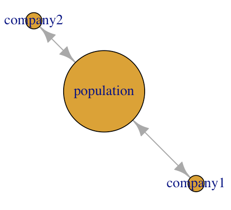
In the following, for all results, I always initialize the simulation scenario as follows:
stocks <- list()
## Let's work with two stocks
## First will be the unemployed population, with "big" capacity to consume/pour flows:
stocks <- add_stock(stocks, stock_name = "population", initial_stock=100, inflow=1000, outflow=1000)

stocks <- add_stock(stocks, stock_name = "company1", initial_stock=20, inflow=3, outflow=2)
stocks <- add_stock(stocks, stock_name = "company2", initial_stock=20, inflow=7, outflow=3)
Each “stock” in turn can evolve with the (discrete) passing of time (how much time will be important as we’ll see in a moment), and I choose to represent that as “in-flows” and “out-flows” volume, which in turn are supposed here to represent the corresponding “policy” of each company.
Again, I’m making stuff up as I go here, so… For instance, I add some randomness to the process (just for the fun of it) so that at time step X, company 1 with inflow 3 would try to “hire” 3 employees, but I add a probability of 40% whereby the company at that particular time-step X decides to hire someone. The same goes for firing (in the case of company 1, the policy says “fire 2”). And all that applies exactly the same for company 2, with its own policy.
So it could look like so:
consume_from_population <- function(stocks, consumer_stock_num) {
    ## Add some level of randomness
    if(runif(1) > 0.4)
        if(stocks[[1]]$current_stock > 0) {
            ## stocks[[1]] is the general population...
            consumable <- min(stocks[[1]]$current_stock, stocks[[consumer_stock_num]]$inflow)
            stocks[[1]]$current_stock <- stocks[[1]]$current_stock - consumable
            stocks[[consumer_stock_num]]$current_stock <- stocks[[consumer_stock_num]]$current_stock + consumable
        }
    stocks
}

...
The general population starts off with 100 individuals, and is not limiting in that it could potentially gather “people” from - or pour into - the companies at a rate much higher than what the companies would do.
Simulating the passing of time
Quite simply, this is the core of the simulation, really:
for(current_time in 1:n_time_steps) {
    ## flows processing: circle through the companies
    for(node_id in sample(2:3, 2, replace = F)) {
        ## SIMPLISTIC, probably BAD, I know
        stocks <- consume_from_population(stocks, node_id)
        stocks <- loose_to_population(stocks, node_id)
    }
    ...
}
Right now, I only throw graph-related code to show current size of each in number of employees:
V(g)$size <- sapply(stocks, \(x) x$current_stock)Pretty basic stuff, very “algorithmic”, and again, not much thinking went into doing this “right”.
This is what it looks like for one simulation then:
Some results
While all the above is pretty simplistic, it does suggest “agent-based modeling” stuff, simulations, etc.
And even for such a simple approach, not realistic in the least, let’s have a look at some conclusions…
Because I added some stochastic parameters in there (the 40% thing), I would need to run several simulations per scenario to get a sense of what really is happening.
Today I’ll focus on how long I run the simulation and the impact of limited general population. It’s not rocket science, really, so let’s break it down.
In all cases, I run one scenario 50 times (and then I’ll use that to average results). In all scenarios I start with the same configuration.
Then I decide to run each scenario a number of steps:
n_time_steps_vec <- c(100, 500, 1000, 5000, 10000)
for(n_time_steps in n_time_steps_vec) {
for(i in 1:50) { ## Let's do this simulation a few times, shall we? MC-like
...
}
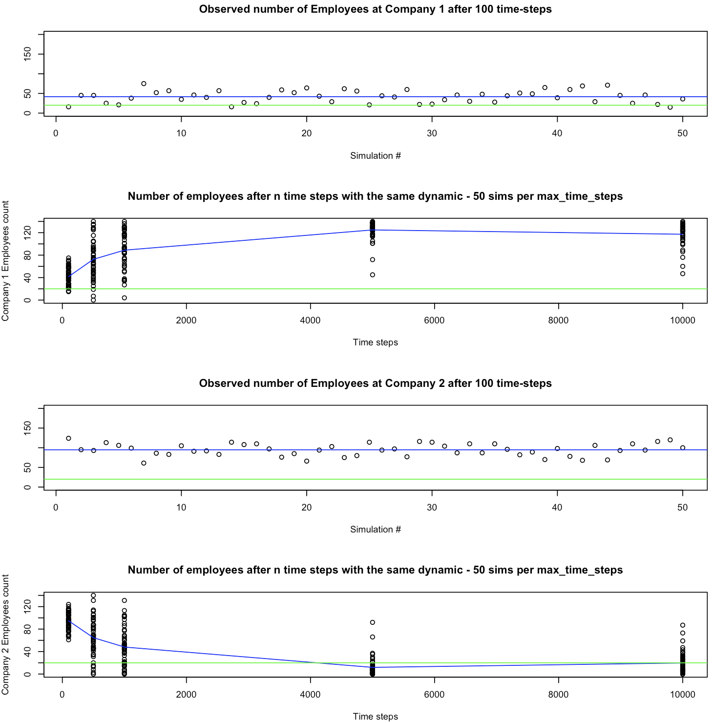
}I’ll show in the next graphics the following, for each company:
After 50 simulations of one scenario, what was the resulting size of the company (in number of employee) in each scenario, when the scenario was run 100 time steps.
Save the resulting 50 simulations per scenario, but run it 100, 500, 1000, 5000 and 10000 time steps. Average (blue line) the resulting size of the company. (Green line: the companies start with 20 employees each)
Show that for both companies (1 on top, 2 at the bottom).
So what does this say?
Well, there is something I am not showing above: The general population!
See, as long as the general population has people to hire, both companies grow, one more than the other, as expected per their respective policies. That is: Company 2 hires even more than it fires people, comparatively, in spite of being less careful with loosing people than Company 1.
However, when the population of candidates is depleted, Company 1, which is less aggressive in hiring but more conservative when it comes to loosing people (i.e. possibly better culture, while maybe less “attractive” to the market “upfront”, say maybe it pays a little less than company 2… Whatever the reason!)…
Right, so when the “general population” is depleted, the policy of the first company pays off!
It makes sense, right? If hiring isn’t an option, well, you better make efforts towards retaining your talent.
Company 1 has a better policy when it directly competes with Company 2 for its resources, instead of consuming from a large pool of candidates.
In other words, if a resource is scarce, and you’re competing directly with others, maybe you should focus on saving that resource, more so than getting more.
And maybe it’s wrong, but this simplistic simulation scenario hints at such a conclusion.
Limitations
Well, to begin with, I don’t know whether my code even makes sense, for example I simply loop through a list of companies, and the “graph” structure really is just used for visualization (maybe I could use some adjacency matrix multiplications instead? Ashby’s Cybernetics book hinted at that… But for states… IDK, right now, no matter).
This is also all very static, too. Both companies stick to their policies no matter what. Not realistic in the least.
And yes, the population is limited. Like a bounded resource. It feels wrong, or at least very incomplete (if that ever happened, people would rush to train themselves to compete to get hired in that market, wouldn’t they?).
Plus, the “40%” decision for hiring/firing at any given time step makes no sense whatsoever, either.
And a long etc. Then again, “all models are wrong”… Well, this one is very wrong. Anyhow, this was just for the fun of the exercise!
Conclusions
I know, too simplistic, not realistic at all. Even poor algorithmic approach, for sure, I don’t know. The goal here was never to go for perfect, but to try out my hand at simulating flows and stocks and a simple interaction scenario.
And yet, some conclusions can come out of it, somewhat in the spirit of “Systems Thinking”.
And that is more than enough for me for now.
It does tell me, once I shift my focus onto a new project for next year (just an idea I have for myself, because I want to work on something that interests me like that, say like the RLCS project these past few months…)… In between ODE and ABM and FSMs, yes…
Yes, maybe that’s where I’ll keep looking for fun stuff to learn.