Migrating to M1, Docker & RStudio included

Intro

So long story short: I’m soon to start working on some reports that will include some math stuff.

I could do that with a Word-like editor, but why would I when we have the marvelous R Markdown? Let’s test a few things that will surely come in handy…

Creating reports to share

So suppose you want to give a human (person) a report for them to use, being able to send it over email, supposing only that that person will be able to open it with a PDF reader. (For a machine, PDFs are awful of course, but for humans well…).

So first, we’ll need to have the capacity to “knit” Rmd files, which comes natively with RStudio (good). However, for PDF, our Docker container by default lacks some stuff, so we’ll have to throw that into our Dockerfile; here is the relevant part of it for this purpose:

RUN apt-get -y install xml2 curl less \
default-jre python3-virtualenv python3-pip \
texlive-base texlive-latex-base texlive-bibtex-extra texlive-fonts-recommended texlive-latex-extra

The third line is what we’ll need to “Knit to PDF” in our container, which in the base rocker/rstudio image wasn’t included.

For reference, the version of Dockerfile I’m using at this point is here.

We can test it directly with a default new .Rmd (choosing PDF as default format) file, and it should work now.

Creating a template

Next up, let’s make sure we create consistent reports over time (say we need to create new reports for the same person every now and then in the future…). A few things come to mind, but let’s keep it simple: We want a title, author, table of contents, and a header logo.

The header logo I needed to lookup as I had no idea how to do it, I landed on this StackOverflow page which led to the following in the header:

header-includes: 
 \usepackage{graphicx}
 \usepackage{fancyhdr}
 \pagestyle{fancy}
 \setlength\headheight{28pt}
 \fancyhead[L]{\includegraphics[width=5cm]{logo_1.png}}
 \fancyfoot[LE,RO]{GPIM}

Provided you have the logo_1.png file in the same folder as the Rmd file, you should be OK.

Then the table of contents, it’s pretty standard stuff, more on that can be found here.

The result header would then look like so:

---
title: "Markdown_template.Rmd"
author: "Your name here"
date: "`r Sys.Date()`"
header-includes: 
 \usepackage{graphicx}
 \usepackage{fancyhdr}
 \pagestyle{fancy}
 \setlength\headheight{28pt}
 \fancyhead[L]{\includegraphics[width=5cm]{logo_1.png}}
 \fancyfoot[LE,RO]{GPIM}
output: 
 pdf_document:
  toc: true
  toc_depth: 2
---

So now we have a basic template we will be able to re-use in future reports, that should help us be a little bit more efficient.

Throwing in some real-looking math

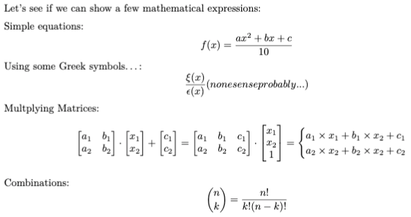
Now we already have loaded LaTeX to our container, so it should be no problem to use it. In R Markdown, you’d use the “$$” signs to begin/end a LaTeX-evaluated expression:

Simple equations:
$$ f(x) = {{ax^2 + bx + c} \over 10}$$

Using some Greek symbols...:
$$ {\xi(x) \over \epsilon(x)} (nonesense \space probably...)$$

Multplying Matrices:
$$ \begin{bmatrix}
a_1 & b_1\\
a_2 & b_2 
\end{bmatrix} \cdot \begin{bmatrix} x_1\\
x_2
\end{bmatrix} + 
\begin{bmatrix} c_1\\
c_2
\end{bmatrix} = 
\begin{bmatrix}
a_1 & b_1 & c_1\\
a_2 & b_2 & c_2
\end{bmatrix} \cdot \begin{bmatrix} x_1\\
x_2\\
1
\end{bmatrix} =
\begin{cases}
a_1 \times x_1 + b_1 \times x_2 + c_1\\
a_2 \times x_2 + b_2 \times x_2 + c_2
\end{cases}$$

Combinations:
$$ {n \choose k} = \frac{n!}{k!(n-k)!} $$

The above code nicely helps us output the following:

Then add some functions plots

For good measure, let’s see how we might go about plotting functions using R (although that might not be needed as I might be pushed into using another language, in which case I’d include screen captures, I guess…).

So here is where I found what I needed for this purpose. I’ll have to read a bit more through it, but it’s looking good. One issue though, the thing I needed here the most was the function slice_plot(), which doesn’t seem to work (even after testing this).

So instead, I went ahead and implemented a simplistic version of it myself:

library(mosaicCore)
library(plyr)
library(ggplot2)
library(gridExtra)

# for better readability:
g <- makeFun(2*x^2 - 5*x + 2 ~ x) # requires mosaicCore

my_function_plotter <- function(in_func, c_range, s_step = 0.1) {
  plot_df <- rbind.fill(lapply(seq(c_range[1], c_range[2], s_step), function(i) {
    data.frame(x = i, f_x = in_func(i))
  } ))

  ggplot(plot_df, aes(x = x, y = f_x)) +
    geom_line()
}

ggp_1 <- my_function_plotter(g, c_range = c(-2, 2), s_step = 1)
ggp_2 <- my_function_plotter(g, c_range = c(-2, 2), s_step = 0.1)

grid.arrange(ggp_1, ggp_2, ncol=2)

With that put into the Rmd, we get to plot a function (in this case with two different “steps”, the smaller the step, the better the resolution:

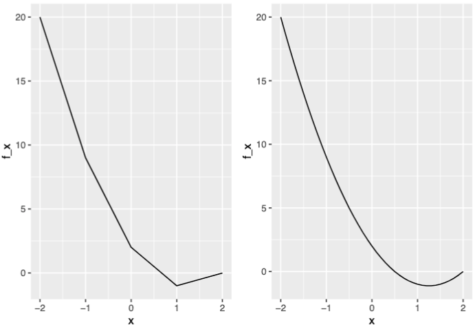
Good enough.

Conclusions

I think I’m about as ready as it gets to start reporting on scientific/mathematical stuff. Which is a good thing, as I’ll need it soon.

And all from our RStudio container!

References

For RMD, https://bookdown.org/yihui/rmarkdown-cookbook

For LaTeX, overleaf and StackExchange for TeX

Calculus with R (mostly to make use of “makeFun()”), https://dtkaplan.github.io/RforCalculus/