RLCS: A (shorter) Introduction

Interpretable, Symbolic Machine Learning

An issue with “AI”: explainability

Let’s call it Machine Learning. As of today:

• Mostly Neural networks, DNN, and that’s all black boxes

There are ways around that.

An issue with “AI”: explainability

Interpretability/Explainability:

• Model-specific Methods (…)

• Local Model-Agnostic Methods: Counterfactuals, Local Surrogate Model (LIME), Shapley Value, Shapley Additive exPlanation (SHAP)…

• Global Model-Agnostic Methods: Partial Dependence Plot (PDP), Accumulated Local Effects (ALE), H-Statistic, Surrogate Models…

• Interpretable Models: Trees, LM/GLM, KNN, and rule-based

Recommended reading: Molnar C. (2022) “Interpretable Machine Learning”

A new R package

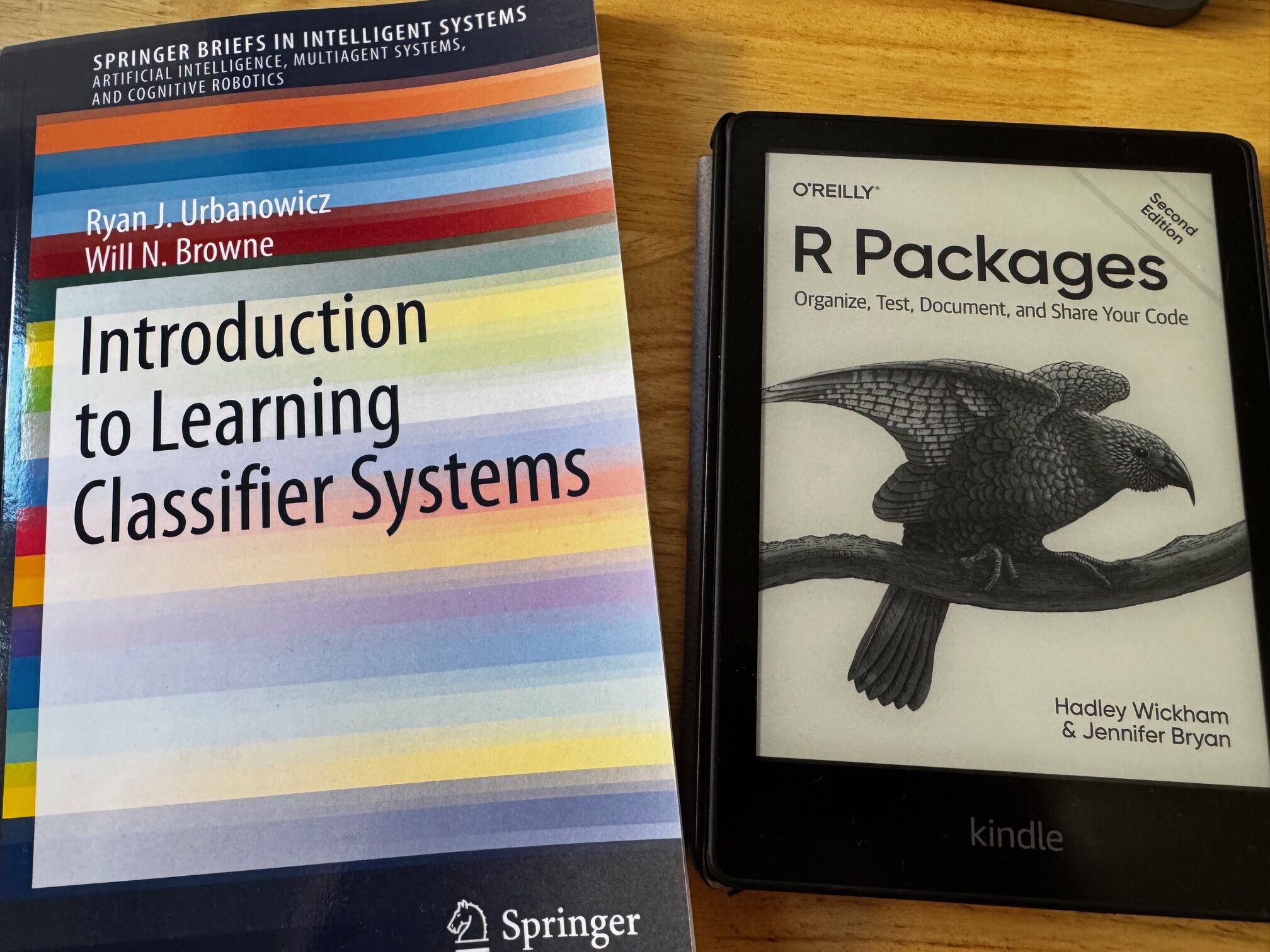
John H. Holland proposed an algorithm with the Cognitive System One program (1976). Later, people came up with variations… Today we focus on Michigan-style LCS.

A preview

Can you guess the “rule”?

A Data Mining Exercise with RLCS

> library(RLCS)
> demo_env1 <- rlcs_example_secret1()
> sample_of_rows <- sample(1:nrow(demo_env1), 10, replace=F)
> print(demo_env1[sample_of_rows,], row.names = F)
 state class
 01010     0
 00111     0
 11010     0
 10001     1
 00010     0
 00100     1
 10100     1
 01111     0
 01100     1
 00001     1

Did you guess right?

> demo_params <- RLCS_hyperparameters(n_epochs = 280, deletion_trigger = 40, deletion_threshold = 0.9)
> rlcs_model1 <- rlcs_train_sl(demo_env1, demo_params, NULL, F)
[1] "Epoch: 40 Progress Exposure: 1280 Classifiers Count: 14"
[1] "Epoch: 80 Progress Exposure: 2560 Classifiers Count: 8"
(...)
[1] "Epoch: 280 Progress Exposure: 8960 Classifiers Count: 2"

Condition/Action is the rule (the rest are quality metrics)

> print(rlcs_model1)
  condition action match_count correct_count accuracy numerosity reward first_seen
1     ###1#      0        3560          3560        1        122      5       1843
2     ###0#      1        2770          2770        1         94      5       3421

This model expresses: “Action/Class is Not bit 4”

Learning rules as model(s)

• if A & NOT(B) then Class=X

• if D then Class=Y

“Human-readable”, “interpretable”, good for:

• Mitigating bias(es) (in training data, at least)

• Increased trust (justifying decisions)

Learning about the data (data mining), better decisions, regulatory compliance, ethical/legal matters, possible adversarial attack robustness…

Interlude: Get the package

Download and install RLCS

https://github.com/kaizen-R/RLCS

To get the package from GitHub:

library(devtools)
install_github("kaizen-R/RLCS")

Run your first test

library(RLCS)
demo_params <- RLCS_hyperparameters(n_epochs = 400, deletion_trigger = 40, deletion_threshold = 0.9)
demo_env2 <- rlcs_example_secret2()
print(demo_env2, row.names = F)
rlcs_model2 <- rlcs_train_sl(demo_env2, demo_params, NULL, F)
print(rlcs_model2)
plot(rlcs_model2)

Binary input: Example

Neural Networks accept numerical input. Currently, RLCS accepts Binary strings.

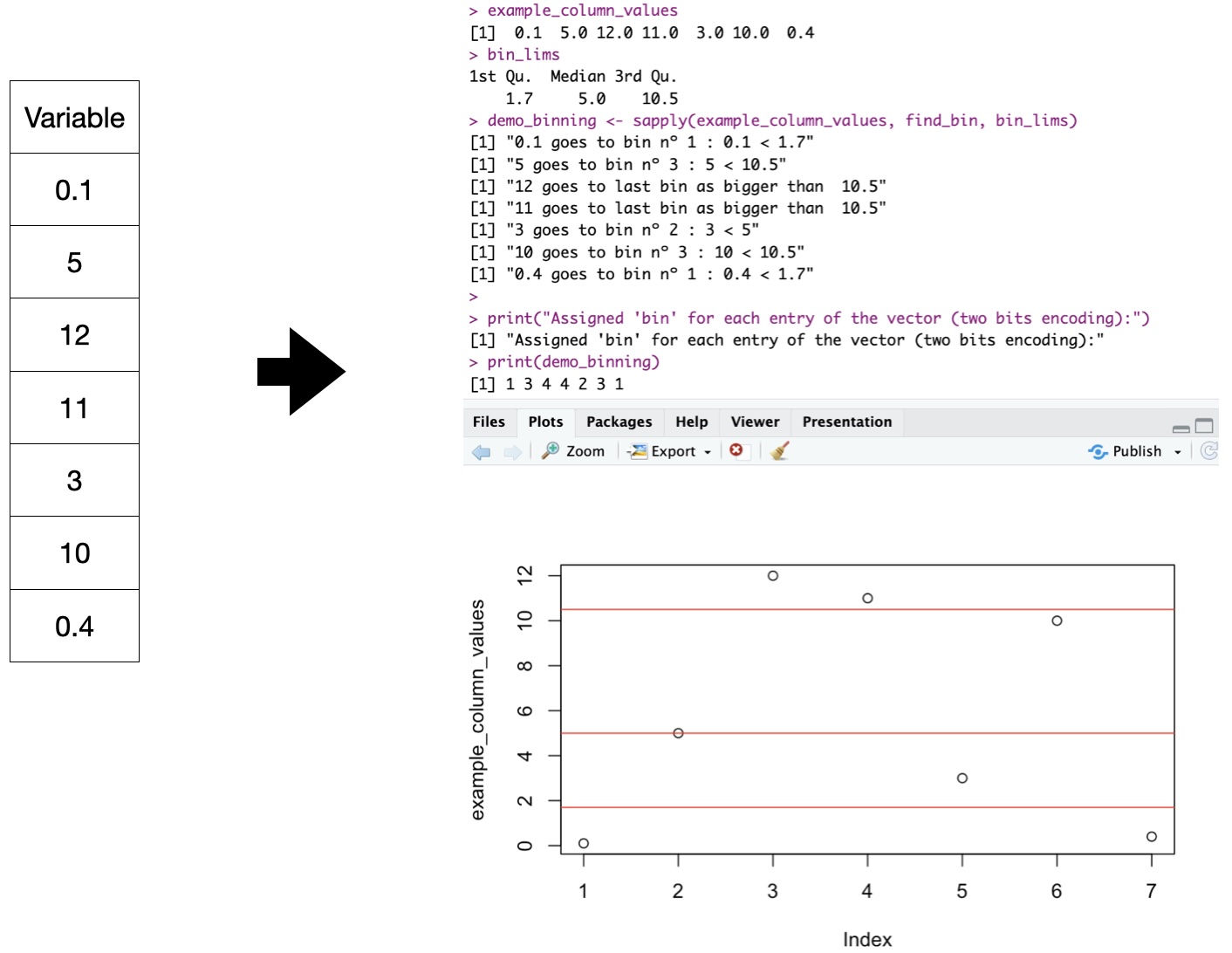
Rosetta Stone “binning” for numerical variables (2 bits explanation)

What can RLCS do?

Data Mining

We’ve seen simple examples. A few more are included with the package, have a look at the demos.

Supervised Learning: Iris

Iris Setosa (https://commons.wikimedia.org/w/index.php?curid=57593826)

Iris Sample Dataset

Time difference of 13.13619 secs ## Training Runtime.
            predicted
class        setosa versicolor virginica
  setosa         13          0         0
  versicolor      0          5         3
  virginica       0          0         9

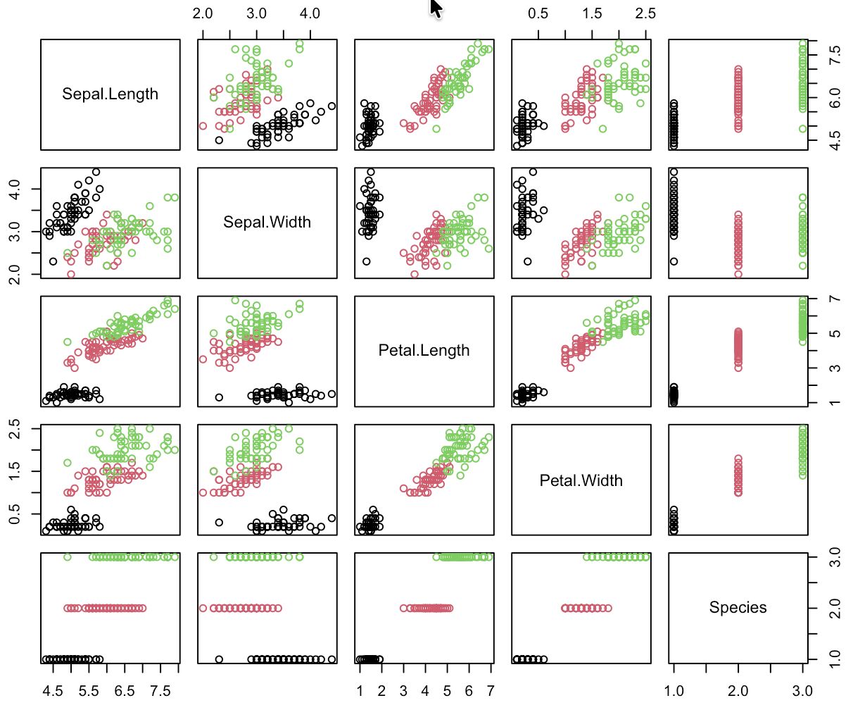
Supervised Learning: Iris

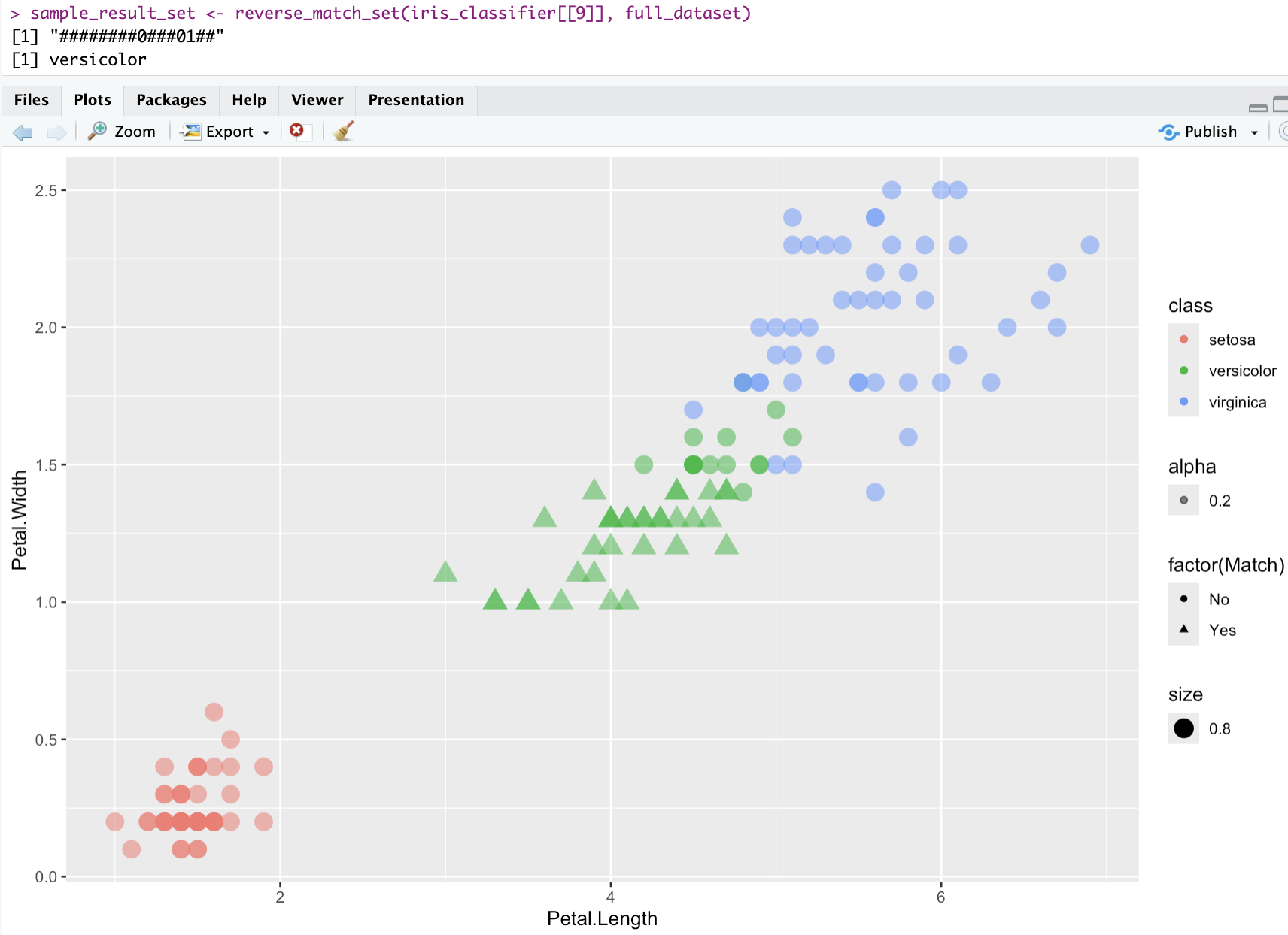
visualizing one classifier - iris

Supervised Learning: Images Classifier

[1] "Accuracy: 0.98"
> table(test_mnist_bin01_49b[, c("class", "predicted")])
     predicted
class    0    1 rlcs_no_match
    0 1716   65             5
    1    5 2008             0
>
> ## Training time on 800 samples:
> print(t_end - t_start)
Time difference of 1.937979 mins

!! Magic Trick: Parallelism: By splitting training data, and then consolidating sub-models! (Take that, Neural network :D)

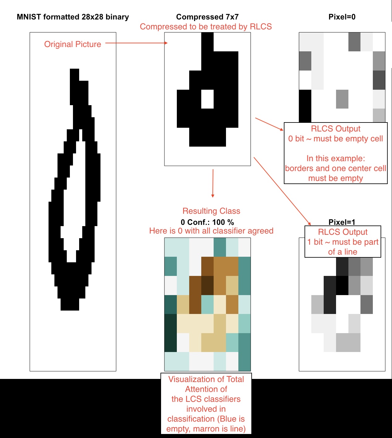
Supervised Learning: Images Classifier

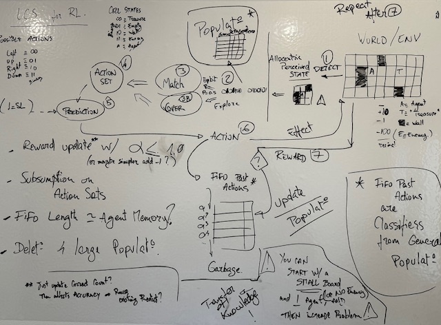
Reinforcement Learning, TOO!

This example is in fact not learning probability distributions. And it uses reward-shaping. But it works!

Then again

Hyperparameters tuning is not easy, and impacts performance. Large Populations of rules are in fact hard to interpret, in spite of being readable.

This is all work in progress. I plan to try and make it into a CRAN Package. (So: document more, write more tests, reorganize functions…) I will keep working on better mechanics (fitness sharing, deletion, etc.), parallel processing, help with encoding/decoding, etc.

More Resources

• THE BEST INTRO to the LCS Algorithm out-there (hands down!) (12’ video)

• Wikipedia on LCS

• Advanced R is ALWAYS great

Thank you!