RLCS: An Introduction

Interpretable, Symbolic Machine Learning

An issue with “AI”: explainability

Let’s call it Machine Learning. As of today:

Mostly Neural networks
And mostly, that means it’s all black boxes

There are ways around that. (e.g. Trees and other “open book” algorithms…)

. . .

John H. Holland proposed an algorithm with the Cognitive System One program (1976). Later, people came up with variations… Today we focus on Michigan-style LCS.

Actually… That’s it. No time to dive deeper here.

Today, we’ll be discussing one such explainable Machine Learning algorithm.

Learning rules as model(s)

if A & NOT(B) then Class=X
if D then Class=Y

. . .

“Human-readable”, “interpretable”, good for:

Mitigating bias(es) (in training data, at least)
Increased trust (justifying decisions)

. . .

Learning about the data (data mining), better decisions, regulatory compliance, ethical/legal matters, possible adversarial attack robustness…

A new R package

. . .

Have you ever found something that no one else has done?

I found such a thing last November 2024. But let’s go back for a minute.

A preview

Can you guess the “rule”?

> library(RLCS)
> demo_env1 <- rlcs_example_secret1()
> sample_of_rows <- sample(1:nrow(demo_env1), 10, replace=F)
> print(demo_env1[sample_of_rows,], row.names = F)
 state class
 01010     0
 00111     0
 11010     0
 10001     1
 00010     0
 00100     1
 10100     1
 01111     0
 01100     1
 00001     1

Did you guess right?

> demo_params <- RLCS_hyperparameters(n_epochs = 280, deletion_trigger = 40, deletion_threshold = 0.9)
> rlcs_model1 <- rlcs_train_sl(demo_env1, demo_params, NULL, F)
[1] "Epoch: 40 Progress Exposure: 1280 Classifiers Count: 14"
[1] "Epoch: 80 Progress Exposure: 2560 Classifiers Count: 8"
[1] "Epoch: 120 Progress Exposure: 3840 Classifiers Count: 2"
[1] "Epoch: 160 Progress Exposure: 5120 Classifiers Count: 2"
[1] "Epoch: 200 Progress Exposure: 6400 Classifiers Count: 2"
[1] "Epoch: 240 Progress Exposure: 7680 Classifiers Count: 2"
[1] "Epoch: 280 Progress Exposure: 8960 Classifiers Count: 2"

. . .

> print(rlcs_model1)
  condition action match_count correct_count accuracy numerosity reward first_seen
1     ###1#      0        3560          3560        1        122      5       1843
2     ###0#      1        2770          2770        1         94      5       3421

The model expresses: “Not bit 4”

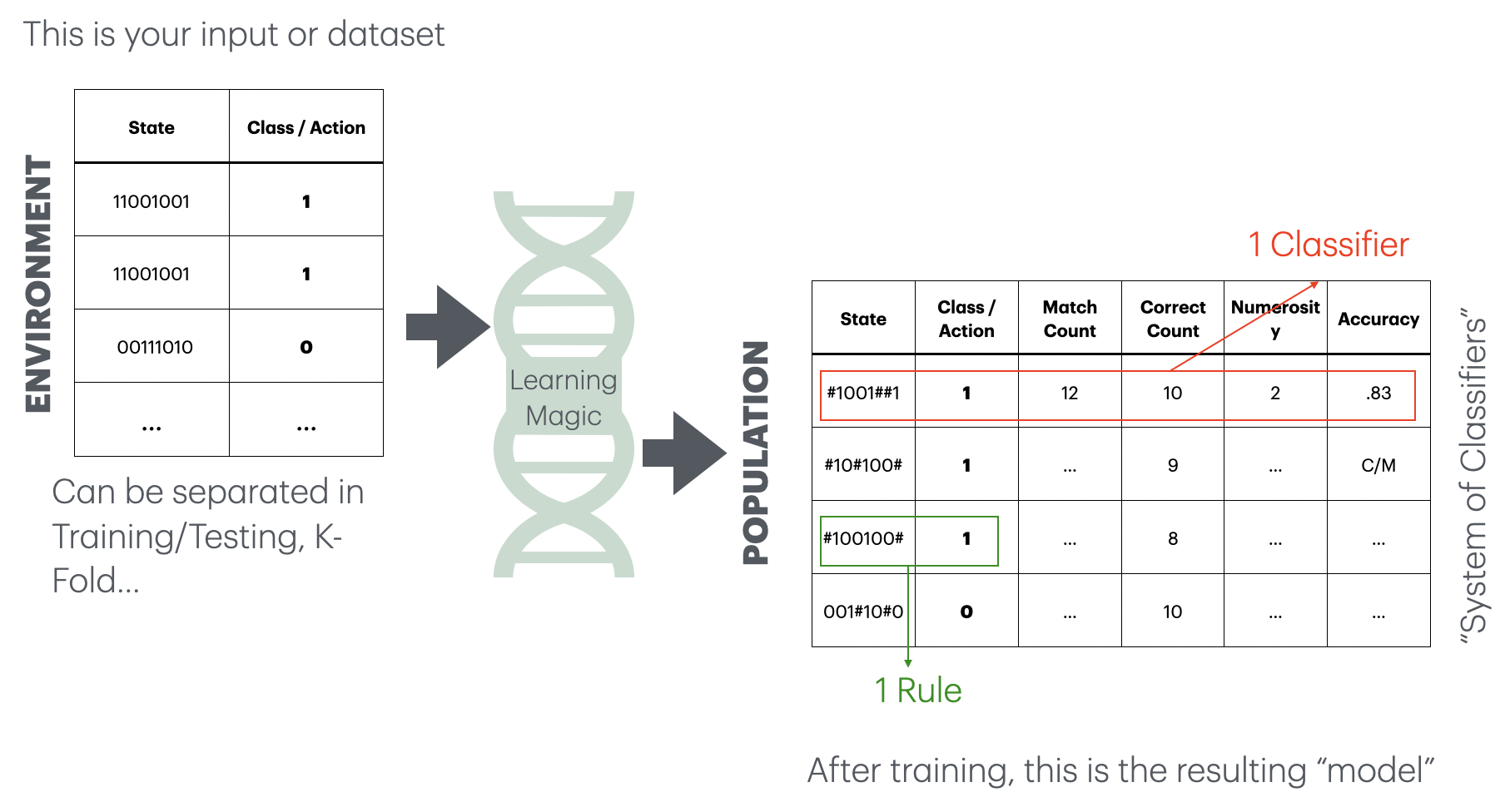
The model: the Ternary Alphabet

A Population of Classifiers is produced.

This is how to read that output model:

Each classifier includes a rule that encodes a match for states that can be read as:

0	No/False/not present
1	Yes/True/present
#	“Don’t care”

RLCS PRE-requisite

The input

Before we dive in:

Neural Networks accept numerical vectors for inputs.

Other algorithms accept factors, or mixed-input.

Well…

. . .

The RLCS package (specific/current implementation) expects binary strings for its input.

The input: Binary encoding

NOTE: This is NOT part of the LCS algorithm per-se.

With the input data, we will encode the data as:

0	No/False/not present/0
1	Yes/True/present/1

A “state” of the environment will then be encoded as a string of zeros and ones.

Binary input?! DO NOT WORRY

Any data point can be encoded into binary strings.

. . .

rlcs_rosetta_stone()

A (simplistic) function is actually provided to make this a bit more transparent. Not necessarily the best approach! Just an “illustration”, really.

(for numerical data, for now… work-in-progress :))

Binary input: Example

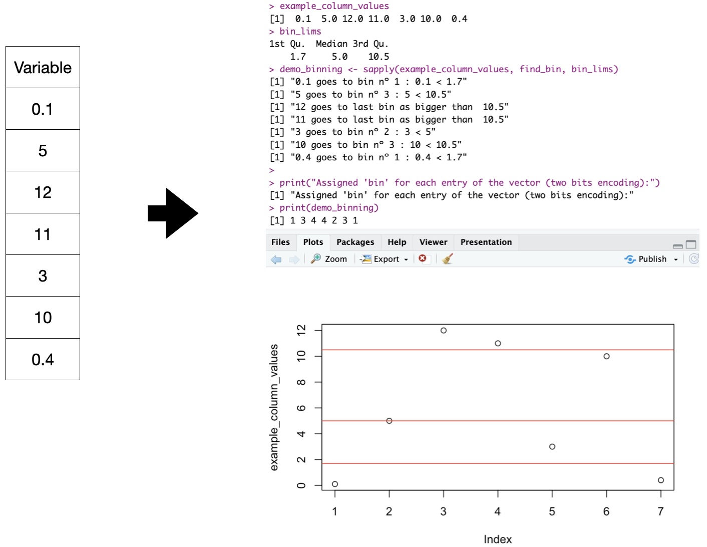
Rosetta Stone “binning” for numerical variables (2 bits explanation)

Binary input: Example

Rosetta Stone: 16 values, 4-bits, “double-quartiles” w/ Gray-binary encoding, per variable:

> head(iris, n=3)
  Sepal.Length Sepal.Width Petal.Length Petal.Width Species
1          5.1         3.5          1.4         0.2  setosa
2          4.9         3.0          1.4         0.2  setosa
3          4.7         3.2          1.3         0.2  setosa
> rlcs_iris <- rlcs_rosetta_stone(iris, class_col=5) ## NOT part of LCS
> head(rlcs_iris$model, n=3)
  rlcs_Sepal.Length rlcs_Sepal.Width rlcs_Petal.Length rlcs_Petal.Width  class            state
1              0010             1111              0011             0010 setosa 0010111100110010
2              0011             0101              0011             0010 setosa 0011010100110010
3              0000             1101              0000             0010 setosa 0000110100000010

Note: with some data loss :S

Interlude: Get the package

Download and install RLCS

To get the package from GitHub:

library(devtools)
install_github("kaizen-R/RLCS")

Run your first tests of RLCS

library(RLCS)
demo_params <- RLCS_hyperparameters(n_epochs = 400, deletion_trigger = 40, deletion_threshold = 0.9)
demo_env2 <- rlcs_example_secret2()
print(demo_env2, row.names = F)
rlcs_model2 <- rlcs_train_sl(demo_env2, demo_params, NULL, F)
print(rlcs_model2)
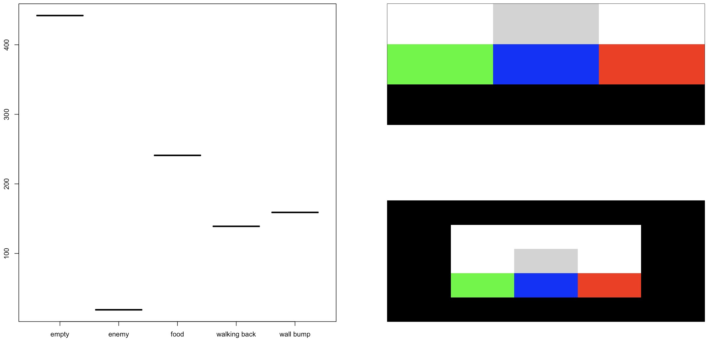
plot(rlcs_model2)

Learning Classifier System: Algorithm

Keywords

Key concepts

1 - Covering

The key: “#” means “I don’t care”

Covering a state with a probability of “#” values means making a rule that matches the input state and class/action.

Something that could match other (partially) similar input:

> generate_cover_rule_for_unmatched_instance('010001', 0.2)
[1] "0#0001"
> generate_cover_rule_for_unmatched_instance('010001', 0.8)
[1] "##0###"

You receive an instance of the environment (a binary string state and a class).

The class here is defined already.

2 - Matching

When you see a new environment instance that does not match any rule in your population yet -> generate a new rule.

. . .

If one(+) rule(s) in your population matches your new instance state -> increase the match count of the corresponding classifier.
If one(+) rule(s) in your population matches your new instance state && class/action –> increase the correct count.

including their corresponding actions

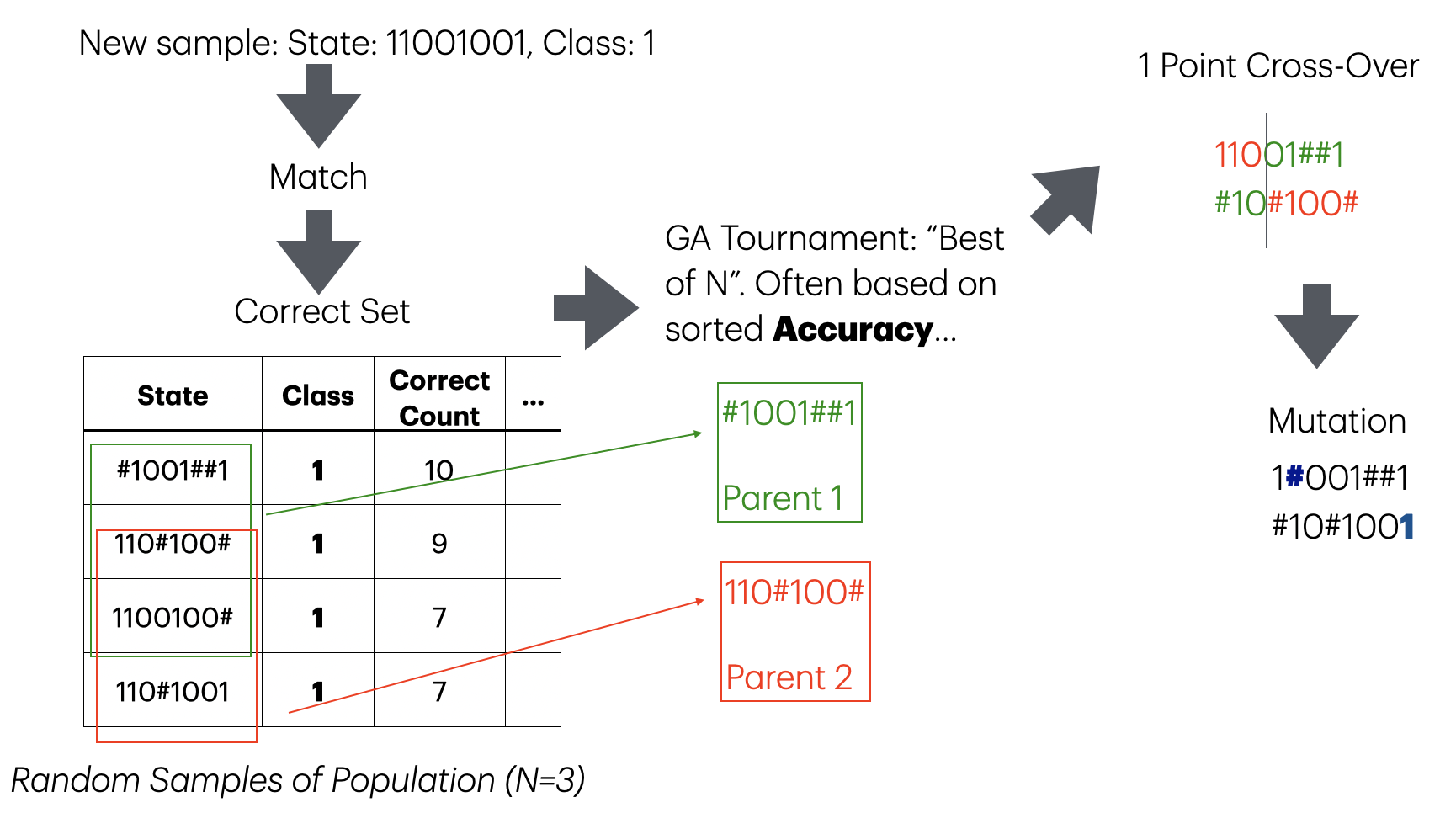
3 - Rule Discovery

After a few epochs of exposing the LCS to your environment, you will have a few rules that match correctly a given instance, the “correct” set.

Match and Correct count are indicators of how good each rule is. But are there other better possibilities?

. . .

Take all the correct set, and apply a Genetic Algorithm to that set, to generate new rules!

3 - Rule Discovery (GA)

mut_point <- which(runif(nchar(t_instance_state)) < mut_prob)

4 - Population Size

Matching must go through all the population every time an environment instance is presented to the LCS.

\[O(match) = epochs*N(environment)*N(population)\]

Where \(N()\) means “size of”.

\[e.g. 1.000 * 5.000 * 1.000 = 5.000.000.000\]

. . .

One option: Reduce the population of rules.

4 - Population Size

Subsumption: A “perfect” classifier that has 100% accuracy might be simpler (more # characters) than other classifiers in the population with same classification. Keep only the best classifiers. (Implemented: Accuracy-based subsumption)
Compaction: You can keep all classifiers that have e.g. 60%+ accuracy after a number of epochs.
Deletion: But you can also cap the population size, keeping only e.g. 10.000 best classifiers.

5 - Prediction

Imagine a new sample/instance, never seen before. (Test environment)

Prediction is about returning the match set for that new instance.

RLCS::get_match_set(sample_state, population_of_classifiers)

. . .

The prediction will be the majority (possibly weighted by numerosity, accuracy…) of the proposed class/action. That’s it! It also means, this is natively an ensemble learning algorithm.

6 - Other uses!

. . .

Why talk about “environment” and “action”? This comes from the world of Reinforcement Learning.

. . .

And because one can read the rules, and “understand” the population, you can also use the LCS to interpret the results and thus do data mining!

All with the same algorithm!

Demo Time

Supervised Learning: Iris

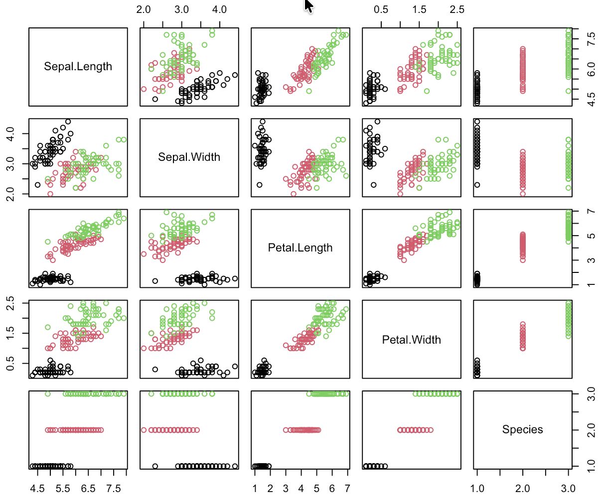
Iris Setosa (https://commons.wikimedia.org/w/index.php?curid=57593826)

Time difference of 13.13619 secs ## Training Runtime.
            predicted
class        setosa versicolor virginica
  setosa         13          0         0
  versicolor      0          5         3
  virginica       0          0         9

Supervised Learning: Iris

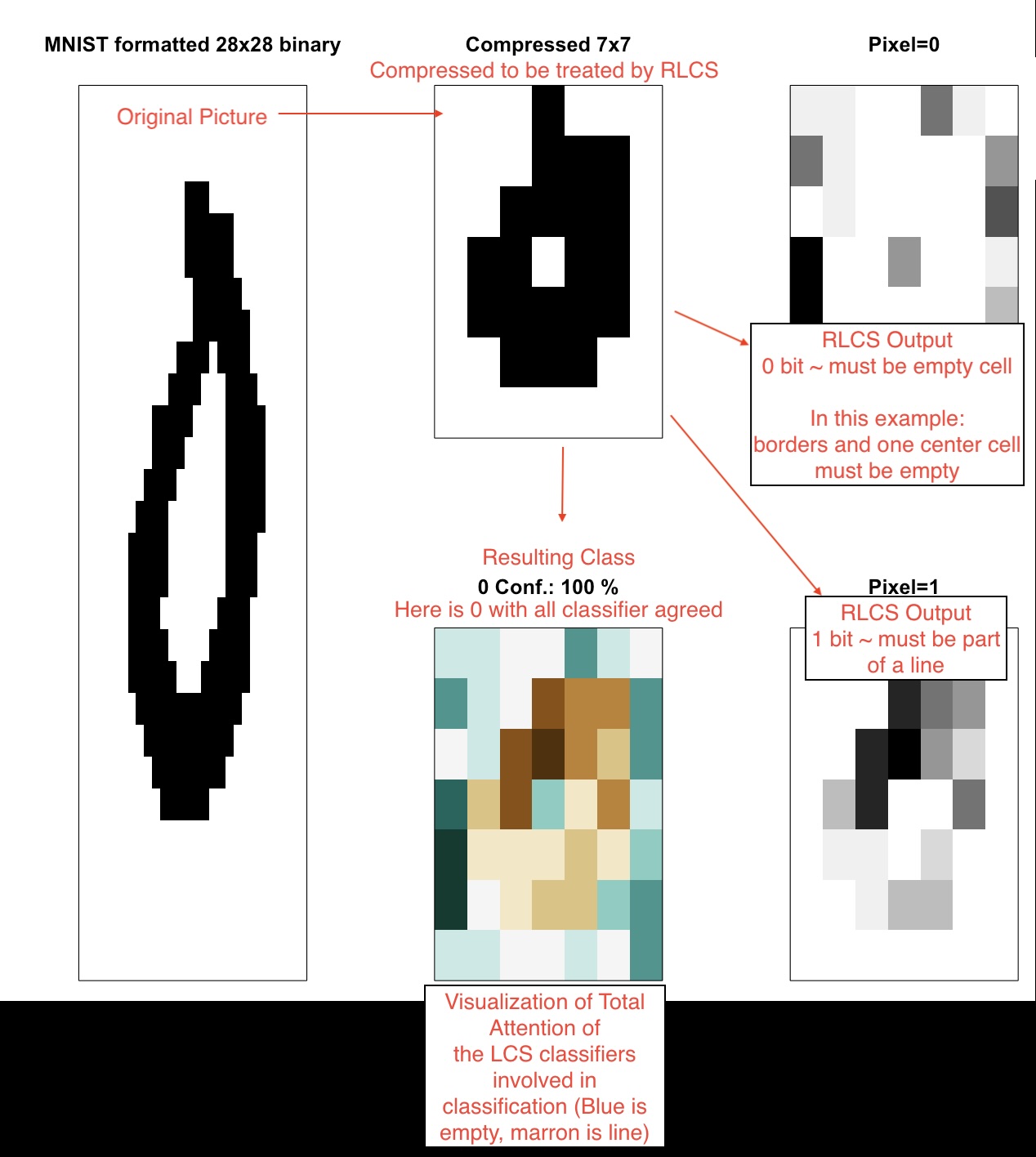
Supervised Learning: Images Classifier

[1] "Accuracy: 0.98"
> table(test_mnist_bin01_49b[, c("class", "predicted")])
     predicted
class    0    1 rlcs_no_match
    0 1716   65             5
    1    5 2008             0
>
> ## Training time on 800 samples:
> print(t_end - t_start)
Time difference of 1.937979 mins

. . .

!! Magic Trick: Parallelism: By splitting training data, and then consolidating sub-models! (Take that, Neural network :D)

Supervised Learning: Images Classifier

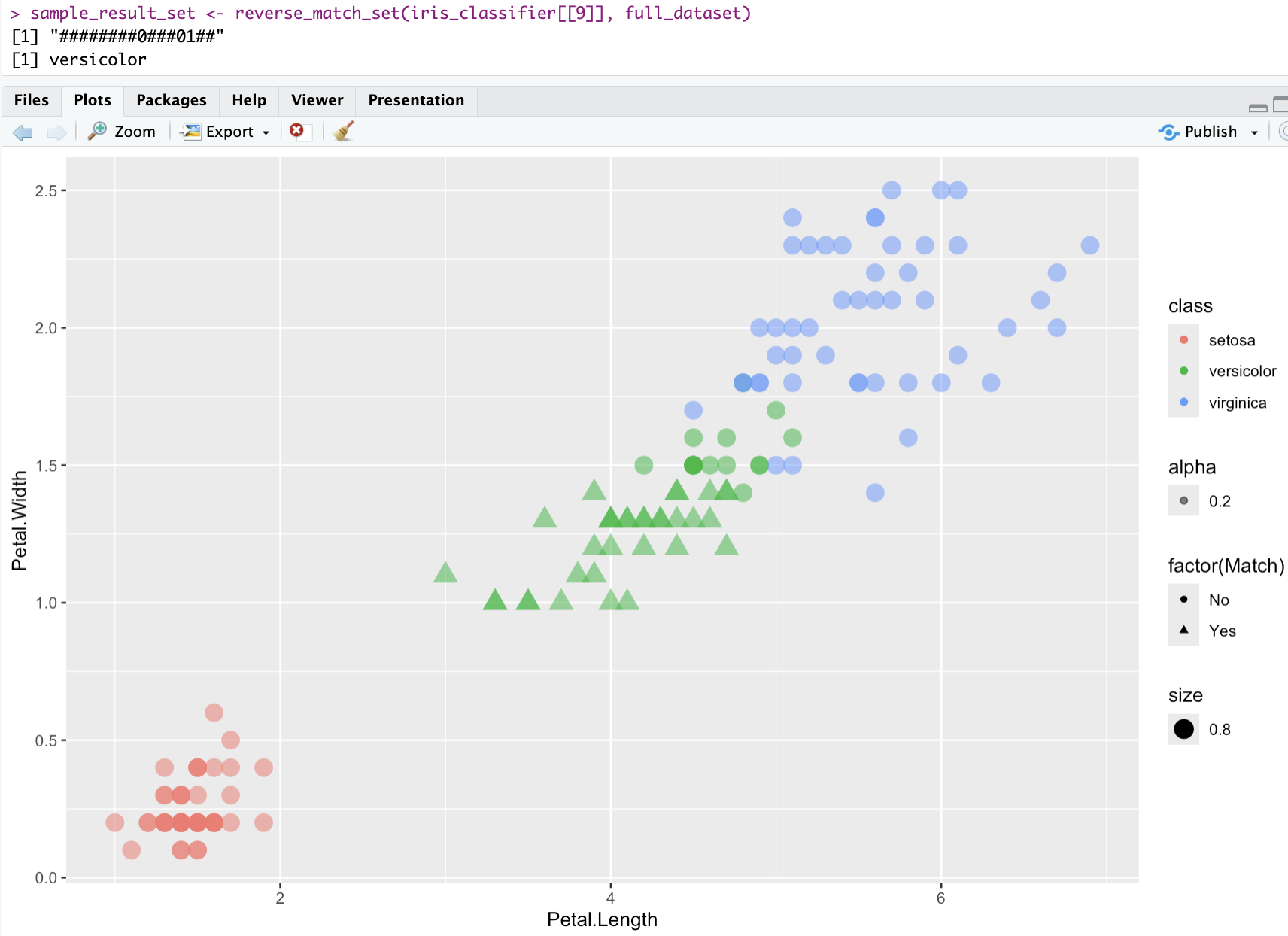
Data Mining

Given that the rules are “expressive”, sometimes you can ask the LCS to find rules that appear in your data:

Not necessarily to classify future samples
To identify what is important for different classes of your data

. . .

REAL WORLD anecdote: inventory of 10K rows with 20 columns, each duly binary encoded. I learnt something about my inventory!

Epistasis

LCS can somehow recognize how two different parts interact. Aptly… The term comes from of genetics (genes modified by other genes…). (e.g. XOR…)

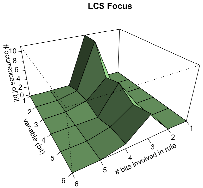
  condition action match_count correct_count accuracy numerosity first_seen
     10##1#      1       15913         15913        1        324        688
     000###      0       15575         15575        1        357       3394
     001###      1       14842         14842        1        298       9231
     11###0      0       13149         13149        1        263      22839
     ...

RL, TOO!

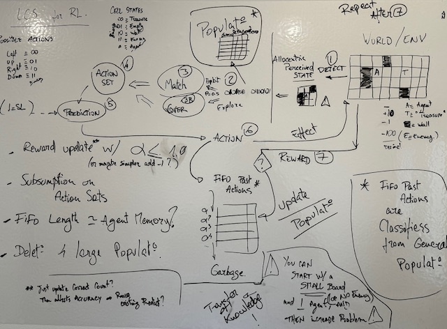
RL Video

Some R code

An R package

A package to implement a simple version of the Learning Classifier System algorithm:

Binary Alphabet, tournament/one-point crossover GA with mutation, accuracy based, Michigan-style LCS
With examples, demonstrating the implementation for:
- Data Mining
- Supervised Learning
- Reinforcement Learning

How did I approach the thing?

Lists. Lists, everywhere. Which might have been a bad idea… (data.table?)
from there, lapply() & al. is then my best friend
“Start small, grow fast” (“fast”… for a hobby, that is)
then clean it (then clean it some more)
Finally publishing on GitHub
Next steps? CRAN

Examples

Before

lcs_res <- rlcs_meta_train(train_environment,
                           1, ## Warmup with just one epoch
                           wildcard_prob,
                           rd_trigger,
                           parents_selection_mode,
                           mutation_probability,
                           tournament_pressure,
                           deletion_trigger) ## Deletion won't be triggered

. . .

Too many parameters! (Uncle Bob wouldn’t like it)

Examples

After, using an object (reference class, “R5”, in this case)

default_lcs_hyperparameters <- RLCS_hyperparameters()
example_lcs <- rlcs_train_sl(train_environment, default_lcs_hyperparameters)

Examples

Or, you know…

source("run_params/datamining_examples_recommended_hyperparameters_v001.R")
basic_hyperparameters <- RLCS_hyperparameters(
  wildcard_prob = wildcard_prob,
  ## defaults for rd_trigger, mutation_probability,
  ## parents_selection_mode && tournament_pressure
  n_epochs = n_epochs,
  deletion_trigger = deletion_trigger,
  deletion_threshold = deletion_threshold
)

## It makes it more readable here:
example_lcs <- rlcs_train(train_environment, basic_hyperparameters)

Examples

Before

inc_match_count <- function(M_pop) { ## All versions
  lapply(M_pop, \(x) {
    x$match_count <- x$match_count + 1
    x
  })
}

inc_correct_count <- function(C_pop) { ## SL Specific
  lapply(C_pop, \(x) {
    x$correct_count <- x$correct_count + 1
    x
  })
}

inc_action_count <- function(A_pop) { ## RL Specific
  lapply(A_pop, \(x) {
    x$action_count <- x$action_count + 1
    x
  })
}

Examples

After, using a function factory

## Function factory to increase parameter counts
inc_param_count <- function(param) {
  param <- as.name(param)
  function(pop) {
    lapply(pop, \(x) {
      x[[param]] <- x[[param]] + 1
      x
    })
  }
}

inc_match_count <- inc_param_count("match_count")
inc_correct_count <- inc_param_count("correct_count")
inc_action_count <- inc_param_count("action_count")

Examples

Before

## Support function for human-compatible printing:
make_pop_printable <- function(classifier) {
    
    df <- plyr::rbind.fill(lapply(1:length(classifier), \(i) {
        t_c <- classifier[[i]]
        data.frame(id = t_c$id,
                   condition = t_c$condition_string,
                   action = t_c$action,
                   match_count = t_c$match_count,
                   correct_count = t_c$correct_count,
                   accuracy = t_c$accuracy,
                   numerosity = t_c$numerosity,
                   first_seen = t_c$first_seen)
    }))
    df[order(df$accuracy, df$numerosity, decreasing = T),]
}

. . .

(Even the parameter name is wrong…)

Examples

After - S3 object

print.rlcs_population <- function(x, ...) {
  if(length(x) == 0) return(NULL)
  x <- .lcs_best_sort_sl(x)
  x <- unclass(x)
  l <- lapply(1:length(x), \(i) {
    t_c <- x[[i]]
    data.frame(condition = t_c$condition_string, action = t_c$action,
               match_count = t_c$match_count, correct_count = t_c$correct_count,
               accuracy = t_c$accuracy, numerosity = t_c$numerosity,
               reward = t_c$total_reward, first_seen = t_c$first_seen)
  })
  # plyr::rbind.fill(l) ## Faster, but adds plyr dependency :(
  ## Slower, but no dependency:
  df <- data.frame(matrix(unlist(l), nrow=length(l), byrow=TRUE))
  names(df) <- c("condition", "action", "match_count", "correct_count", "accuracy", "numerosity", "reward", "first_seeen")
  df
}

. . .

print(example_lcs_population)

Then again

This is all work in progress.

. . .

I plan to make it into a CRAN Package.

So: document more, write more tests, reorganize functions…

More Resources

THE BEST INTRO to the LCS Algorithm out-there (hands down!) (12’ video)
Advanced R is ALWAYS great
And for my first RevealJS Quarto, this blog entry (not mine)
Probably quite a few more, including the two in the first picture.

Follow the link at the bottom for more info!

Thank you!

Supplementary

Why nobody has done it yet?

It’s not fast

There are many sequential steps, rather unavoidable ones at that
Not ideal to compete with a world of GPUs and parallel processing (yet ;))

. . .

It’s “complex”

Or so does the Wikipedia entry say…
When it comes to “alphabets”, it does get messy, I’ll admit

Execution Speed

For instance, this is a “slow” algorithm. Option: Rcpp for Matching

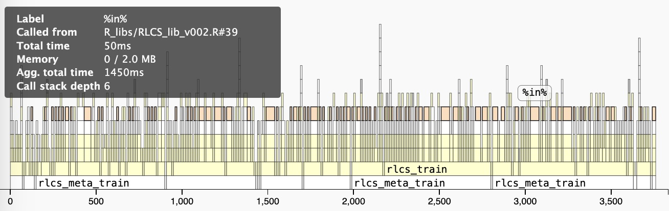
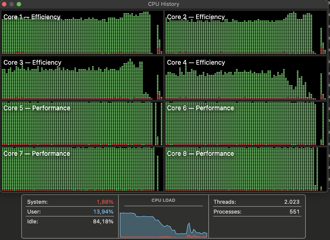
Parallel Computing

Parallel computing? %dopar%, mirai were tested (it all works, but…)

vertical and horizontal partitioning
- Break data set (vertical). Two options
  - instances subsets (reduce population covered per thread/core)
  - Substrings of states (reduce search space)
  - both are “risky”!
- run fewer iterations (epochs) on full dataset, but on several cores in parallel

Parallel Computing

Depending on the dataset, it can be done… Or not…

Reinforcement Learning Conundrum

We’ve seen it works, but… How do you package an RL algorithm?

. . .

You must make assumptions about the “world” your agent is going to interact with. This makes things complicated:

What to include inside the package? What not?
What to expose from the package? What not?

And a few other such questions slow me down a bit…

Other Formats

An issue with “AI”: explainability

Learning rules as model(s)

A new R package

A preview

Can you guess the “rule”?

Did you guess right?

The model: the Ternary Alphabet

RLCS PRE-requisite

The input

The input: Binary encoding

Binary input?! DO NOT WORRY

Binary input: Example

Binary input: Example

Interlude: Get the package

Download and install RLCS

Run your first tests of RLCS

Learning Classifier System: Algorithm

Keywords

Key concepts

1 - Covering

2 - Matching

3 - Rule Discovery

3 - Rule Discovery (GA)

4 - Population Size

4 - Population Size

5 - Prediction

6 - Other uses!

Demo Time

Supervised Learning: Iris

Supervised Learning: Iris

Supervised Learning: Images Classifier

Supervised Learning: Images Classifier

Data Mining

Epistasis

RL, TOO!

RL Video

Some R code

An R package

How did I approach the thing?

Examples

Examples

Examples

Examples

Examples

Examples

Examples

Then again

More Resources

Follow the link at the bottom for more info!

Thank you!

Supplementary

Why nobody has done it yet?

Execution Speed

Parallel Computing

Parallel Computing

Reinforcement Learning Conundrum